2. A Gentle Introduction to DAGs for Bayesian Models#
In this unit, we begin our exploration of Bayesian models. In the second half of the course, we will implement these models using PyMC. Before diving into code, however, we must first introduce some foundational concepts that allow us to express Bayesian models precisely. Among the most essential tools for this purpose are ideas from graph theory.
What is a Graph?#
A graph is a collection of nodes (sometimes called vertices) and the edges that connect them. It’s helpful to think of a node as representing an entity, and an edge as representing a relationship or interaction between two entities:
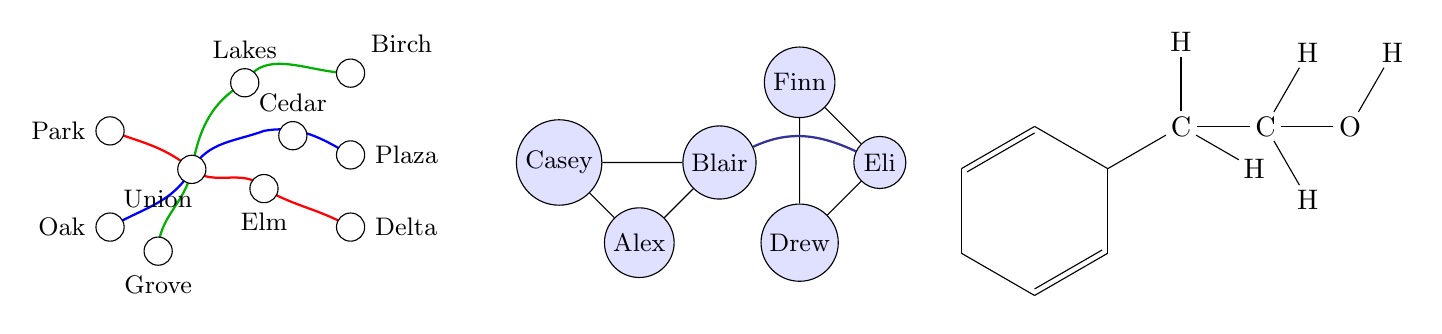
Examples of Graphs: Left: a transit map; Center: a social network; Right: a molecular structure (2-phenylethanol). Each is an everyday construct that can be represented as a graph—a set of nodes and edges.
Graphs come in two main forms:
An undirected graph has edges with no direction. If there is an edge between nodes \(A\) and \(B\), we write \(A\)–\(B\), and the relationship is symmetric. These types of graphs are often used to represent mutual relationships. Think of ‘friendships’ in a social network.
A directed graph (digraph) has edges that point from one node to another. Using social media as an example, with nodes \(A\) and \(B\) here are some ways we could write relationships between them:
\(A\rightarrow B\) : Person \(A\) follows person \(B\), but person \(B\) does not follow person \(A\).
\(B\rightarrow A\) : Person \(B\) follows person \(A\), but person \(A\) does not follow person \(B\).
\(A\leftrightarrow B\) : \(A\) and \(B\) are friends with each other
Each of these can also be cyclic or acyclic:
A cyclic graph contains at at least one path that allows you to start at a node and return to the same place. Using websites as an example: If Site \(A\) links to Site \(B\), Site \(B\) links to Site \(C\), and Site \(C\) links back to Site \(A\), that forms a cycle.
An acyclic graph has no cycles. You cannot return to a starting point by following a sequence of edges.
Bayesian Models as Graphs:#
Bayesian models are expressible as Directed Acyclic Graphs (DAGs). We have previously seen some simple Bayes networks where the nodes are events. Now, the nodes represent the random variables in the model and edges denote the statistical dependencies between the nodes.
Why Graphs? Why DAGs?#
Nodes and edges are a useful way to track the relationships between variables and the dependence structure of your model. The absence of an edge between nodes means there is no direct dependence between those random variables. This method is intuitive and compact but also allows us to leverage the Markovian property. This is useful in inference later.
Consider first the graph (U6 L1 Video, 4:23 , Lecture Slide #5 in PDF) \(A\rightarrow B \rightarrow C\)
Each arrow between nodes encodes a conditional dependence:
\(B\) depends on \(A\).
\(C\) depends on \(B\)
Therefore \(B\) influences \(C\)
Note that \(A\) cannot directly influence \(C\). It can only influence \(C\) through \(B\). This structure has important implicatons for how we factor the joint distribution \(P(A,B,C)\).
Recall that the chain rule (or general product rule) allows us to decompose the joint probability into a product of conditional probabilities:
Connecting this to the Markov Property:#
In the context of our Bayesian models, the Markov property states that a node is conditionally independent of the node’s non-descendants given the node’s parents. Applied to our graph:
Explanations: |
Graph \(A\rightarrow B \rightarrow C\): |
|---|---|
Parent(s) |
Variable \(A\) |
Descendants |
Variable B |
Non-descendants |
Variable C |
Note that for node \(C\), the Markov property applies: \(C \perp\!\!\!\perp A \vert B\). We take this as ground truth and proceed to show something interesting about \(A\). We can prove that even though we are conditioning on \(B\) and \(C\), the additional information from \(C\) is redundant once \(B\) is known. We can do this using only Bayes’ Rule, Conditional Probability, and the chain rule from above: Consider \(P(A\vert B,C)\):
Applying both the Markov Property and the chain rule gives us:
What we have observed here is a simple case of \(d\)-separation: a graphical criterion that determines when two sets of nodes are conditionally independent, given a third set.