3. Priors with Structural Information

This page contributed by Jason Naramore!

An example model is defined with a Binomial likelihood and several hierarchical priors:

\[\begin{split}\begin{align*} X | p & \sim \text{Bin}(n,p) \\ p | k & \sim \text{Beta} (k,k) \\ k | r & \sim \text{Geom}(r), p(k=i) = (1-r)^{i-1} r,\space i = 1,2,... \space \space 0<r<1 \\ r & \sim \text{Beta}(2,2) \\ \end{align*} \end{split}\]

It is expected that \(p\) should be around 0.5, so the prior on \(p\) is set with \(\alpha = \beta\), since the mean of a Beta distribution is \(k / (k+k) = 0.5\). Lower values of \(k\) result in a wider Beta distribution, while higher values of \(k\) result in a tigher distribution.

The idea is that structural information is contained in the \(p | k \sim \text{Beta} (k,k)\), while priors on \(k\) and \(r\) contain subjective information, which could informative or non-informative.

We can build this model in PyMC:

import pymc as pm
import arviz as az
import matplotlib.pyplot as plt
import numpy as np

with pm.Model() as m:
    # priors
    r = pm.Beta("r", 2, 2)
    k = pm.Geometric("k", r)
    p = pm.Beta("p", k, k)

    # likelihood
    x = pm.Binomial("likelihood", p=p, n=5, observed=3)

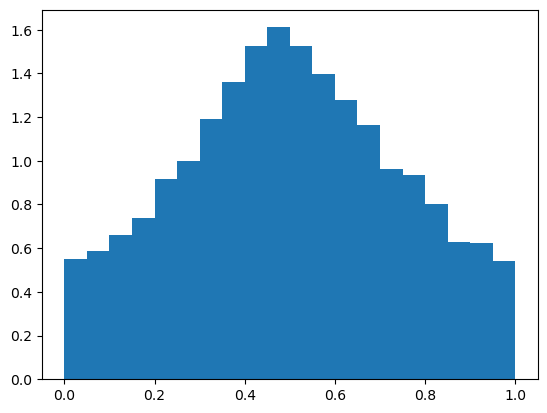
First, let’s sample from the prior predictive and create a histogram of \(p\) before incorporating new data (matching the theoretical plot in the lecture slides):

with m:
    trace_prior = pm.sample_prior_predictive(20000)
az.summary(trace_prior)

Sampling: [k, likelihood, p, r]
arviz - WARNING - Shape validation failed: input_shape: (1, 20000), minimum_shape: (chains=2, draws=4)

	mean	sd	hdi_3%	hdi_97%	mcse_mean	mcse_sd	ess_bulk	ess_tail	r_hat
r	0.501	0.224	0.108	0.901	0.002	0.001	19582.0	19436.0	NaN
k	2.946	6.119	1.000	8.000	0.044	0.031	19978.0	19825.0	NaN
p	0.499	0.243	0.058	0.947	0.002	0.001	19934.0	19936.0	NaN

plt.hist(trace_prior.prior["p"].to_numpy().T, density=True, bins=20)
plt.show()

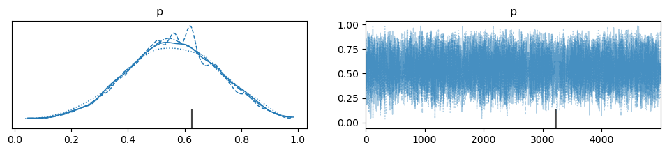
Next, we can sample the posterior distribution. Incorporating the new datapoint of 3/5 successes results in a Bayes estimate in the posterior distribution of \(\approx 0.55\), vs. the MLE of 0.6.

with m:
    trace = pm.sample(5000)
az.summary(trace, hdi_prob=0.95)

Multiprocess sampling (4 chains in 4 jobs)
CompoundStep
>NUTS: [r, p]
>Metropolis: [k]

100.00% [24000/24000 00:01<00:00 Sampling 4 chains, 3 divergences]

Sampling 4 chains for 1_000 tune and 5_000 draw iterations (4_000 + 20_000 draws total) took 2 seconds.
There were 3 divergences after tuning. Increase `target_accept` or reparameterize.

	mean	sd	hdi_2.5%	hdi_97.5%	mcse_mean	mcse_sd	ess_bulk	ess_tail	r_hat
k	3.090	4.111	1.000	10.000	0.227	0.170	691.0	471.0	1.01
r	0.486	0.223	0.089	0.895	0.005	0.004	1559.0	938.0	1.00
p	0.557	0.158	0.260	0.873	0.001	0.001	13095.0	11443.0	1.00

az.plot_trace(trace, var_names="p")
plt.show()

%load_ext watermark
%watermark -n -u -v -iv -p pytensor

Last updated: Mon Jul 29 2024

Python implementation: CPython
Python version       : 3.11.8
IPython version      : 8.22.2

pytensor: 2.18.6

pymc      : 5.11.0
numpy     : 1.26.4
matplotlib: 3.8.3
arviz     : 0.17.1