import pymc as pm
import numpy as np
import arviz as az
import pandas as pd
from pytensor.tensor.subtensor import set_subtensor
import pytensor.tensor as pt
import matplotlib.pyplot as plt

7. Prediction of Time Series*

Adapted from Unit 10: sunspots.odc.

Data can be found here.

Problem statement

Sunspot numbers observed each year from 1770 to 1869.

BUGS Book Page 258.

y = np.loadtxt("../data/sunspots.txt")

y

array([100.8,  81.6,  66.5,  34.8,  30.6,   7. ,  19.8,  92.5, 154.4,
       125.9,  84.8,  68.1,  38.5,  22.8,  10.2,  24.1,  82.9, 132. ,
       130.9, 118.1,  89.9,  66.6,  60. ,  46.9,  41. ,  21.3,  16. ,
         6.4,   4.1,   6.8,  14.5,  34. ,  45. ,  43.1,  47.5,  42.2,
        28.1,  10.1,   8.1,   2.5,   0. ,   1.4,   5. ,  12.2,  13.9,
        35.4,  45.8,  41.1,  30.4,  23.9,  15.7,   6.6,   4. ,   1.8,
         8.5,  16.6,  36.3,  49.7,  62.5,  67. ,  71. ,  47.8,  27.5,
         8.5,  13.2,  56.9, 121.5, 138.3, 103.2,  85.8,  63.2,  36.8,
        24.2,  10.7,  15. ,  40.1,  61.5,  98.5, 124.3,  95.9,  66.5,
        64.5,  54.2,  39. ,  20.6,   6.7,   4.3,  22.8,  54.8,  93.8,
        95.7,  77.2,  59.1,  44. ,  47. ,  30.5,  16.3,   7.3,  37.3,
        73.9])

t = np.array(range(100))
yr = t + 1770

Model 1

with pm.Model() as m1:

    eps_0 = pm.Normal("eps_0", 0, tau=0.0001)

    theta = pm.Normal("theta", 0, tau=0.0001)
    c = pm.Normal("c", 0, tau=0.0001)
    sigma = pm.Uniform("sigma", 0, 100)
    tau = 1 / (sigma**2)

    _m = c + theta * pt.roll(y, shift=-1)[:-1]
    m = set_subtensor(_m[0], y[0] - eps_0)

    _eps = y - m
    eps = set_subtensor(_eps[0], eps_0)

    pm.Normal("likelihood", mu=m, tau=tau, observed=y[:-1])

    trace = pm.sample(3000)

Show code cell output Hide code cell output

Auto-assigning NUTS sampler...
Initializing NUTS using jitter+adapt_diag...
Multiprocess sampling (4 chains in 4 jobs)
NUTS: [eps_0, theta, c, sigma]
/Users/aaron/mambaforge/envs/pymc/lib/python3.11/multiprocessing/popen_fork.py:66: RuntimeWarning: os.fork() was called. os.fork() is incompatible with multithreaded code, and JAX is multithreaded, so this will likely lead to a deadlock.
  self.pid = os.fork()

/Users/aaron/mambaforge/envs/pymc/lib/python3.11/multiprocessing/popen_fork.py:66: RuntimeWarning: os.fork() was called. os.fork() is incompatible with multithreaded code, and JAX is multithreaded, so this will likely lead to a deadlock.
  self.pid = os.fork()

Sampling 4 chains for 1_000 tune and 3_000 draw iterations (4_000 + 12_000 draws total) took 3 seconds.

az.summary(trace)

	mean	sd	hdi_3%	hdi_97%	mcse_mean	mcse_sd	ess_bulk	ess_tail	r_hat
eps_0	-0.014	21.310	-40.006	39.924	0.209	0.201	10412.0	7932.0	1.0
theta	0.817	0.060	0.710	0.937	0.001	0.000	8147.0	7845.0	1.0
c	8.501	3.579	1.758	15.201	0.040	0.029	8081.0	7731.0	1.0
sigma	21.953	1.595	19.064	24.962	0.015	0.011	10940.0	8973.0	1.0

Model 1 using built in AR(1)

with pm.Model() as m1_ar:

    rho = pm.Normal(
        "rho", 0, tau=0.0001, shape=2
    )  # shape of rho determines AR order
    sigma = pm.Uniform("sigma", 0, 100)

    # constant=True means rho[0] is the constant term (c from BUGS model)
    pm.AR("likelihood", rho=rho, sigma=sigma, constant=True, observed=y)

    trace = pm.sample(3000)

Show code cell output Hide code cell output

/Users/aaron/mambaforge/envs/pymc/lib/python3.11/site-packages/pymc/distributions/timeseries.py:621: UserWarning: Initial distribution not specified, defaulting to `Normal.dist(0, 100, shape=...)`. You can specify an init_dist manually to suppress this warning.
  warnings.warn(
Auto-assigning NUTS sampler...
Initializing NUTS using jitter+adapt_diag...
Multiprocess sampling (4 chains in 4 jobs)
NUTS: [rho, sigma]
/Users/aaron/mambaforge/envs/pymc/lib/python3.11/multiprocessing/popen_fork.py:66: RuntimeWarning: os.fork() was called. os.fork() is incompatible with multithreaded code, and JAX is multithreaded, so this will likely lead to a deadlock.
  self.pid = os.fork()

/Users/aaron/mambaforge/envs/pymc/lib/python3.11/multiprocessing/popen_fork.py:66: RuntimeWarning: os.fork() was called. os.fork() is incompatible with multithreaded code, and JAX is multithreaded, so this will likely lead to a deadlock.
  self.pid = os.fork()

Sampling 4 chains for 1_000 tune and 3_000 draw iterations (4_000 + 12_000 draws total) took 2 seconds.

az.summary(trace)

	mean	sd	hdi_3%	hdi_97%	mcse_mean	mcse_sd	ess_bulk	ess_tail	r_hat
rho[0]	8.721	3.572	2.070	15.458	0.049	0.036	5346.0	5707.0	1.0
rho[1]	0.808	0.060	0.694	0.920	0.001	0.001	5248.0	5349.0	1.0
sigma	21.814	1.601	18.806	24.781	0.019	0.013	7213.0	7306.0	1.0

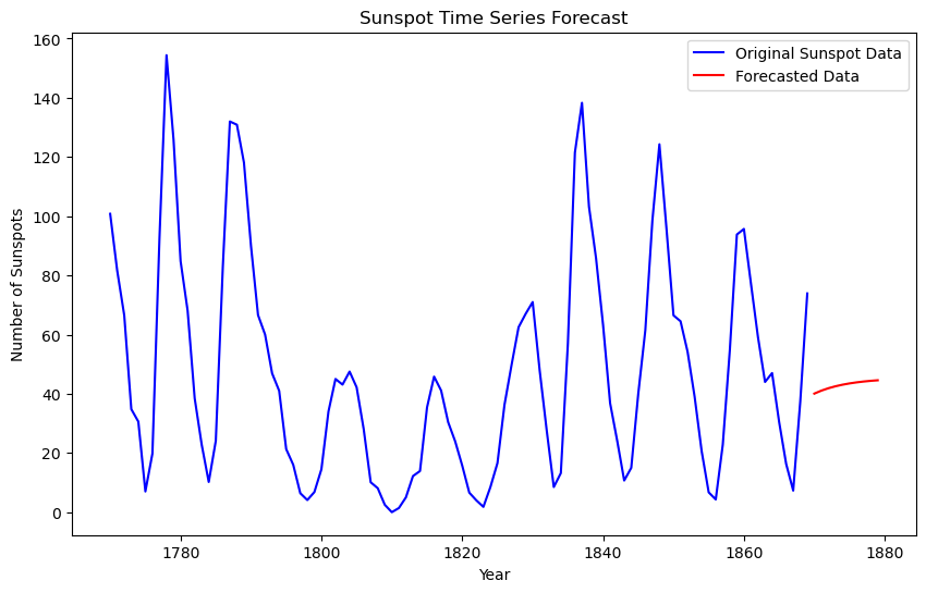
Prediction Step

We have our model, now we forecast the next 10 years:

# Forecast 10 years ahead
n_fcast = 10
y_fcast = np.zeros(n_fcast + 2)
y_fcast[:2] = y[-2:]

# Extract the mean of the posterior for rho (AR(1) model)
rho_mean = trace.posterior["rho"].mean(axis=(0, 1)).values

# Forecast based on the last observed point for AR(1)
for i in range(1, n_fcast + 2):
    y_fcast[i] = rho_mean[0] + rho_mean[1] * y_fcast[i - 1]

y_forecast = y_fcast[2:]

# Extend the year array for the forecast period
t_fcast = np.arange(yr[-1] + 1, yr[-1] + 1 + n_fcast)

# Plot the original time series with the forecast

plt.figure(figsize=(10, 6))
plt.plot(yr, y, label="Original Sunspot Data", color="blue")
plt.plot(t_fcast, y_forecast, label="Forecasted Data", color="red")
plt.xlabel("Year")
plt.ylabel("Number of Sunspots")
plt.legend()
plt.title("Sunspot Time Series Forecast")
plt.show()

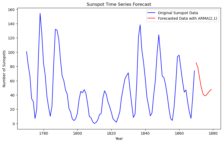
Model 2: ARMA(2,1)

Because the forecast only utilizes the last value to forecast, we will enhance the model by adding another AR term, as well as a Moving Average (MA) term.

We use pymc_experimental.BayesianSARIMA to achieve this. As of 9/16/2024, this functionality is still in the experimentation repo, however it allows for a greatly reduced codebase. Coding an ARMA(2,1) method from scratch is lengthy. See here for documentation.

import pymc_experimental.statespace as pmss
import pymc as pm
import pymc.sampling_jax as pjax

# As BayesianSARIMA does not include an intercept term,
# we can force it by centering the data

y_mean = y.mean()
y_centered = y - y_mean
y2 = y_centered.reshape(-1, 1)

# ARMA(2,1) model
ss_mod = pmss.BayesianSARIMA(order=(2, 0, 1), verbose=True)

with pm.Model(coords=ss_mod.coords) as arma_model:

    # Priors
    state_sigmas = pm.Uniform(
        "sigma_state", 0, 100, dims=ss_mod.param_dims["sigma_state"]
    )
    ar_params = pm.Normal(
        "ar_params", 0, tau=0.0001, dims=ss_mod.param_dims["ar_params"]
    )
    ma_params = pm.Normal(
        "ma_params", 0, tau=0.0001, dims=ss_mod.param_dims["ma_params"]
    )

    # Build Statespace Model
    ss_mod.build_statespace_graph(y2, mode="JAX")

    # Inference Data
    trace = pm.sample(nuts_sampler="numpyro", target_accept=0.9)

Show code cell output Hide code cell output

The following parameters should be assigned priors inside a PyMC model block: 
	ar_params -- shape: (2,), constraints: None, dims: ('ar_lag',)
	ma_params -- shape: (1,), constraints: None, dims: ('ma_lag',)
	sigma_state -- shape: None, constraints: Positive, dims: ()
/Users/aaron/mambaforge/envs/pymc/lib/python3.11/site-packages/pymc_experimental/statespace/utils/data_tools.py:74: UserWarning: No time index found on the supplied data. A simple range index will be automatically generated.
  warnings.warn(NO_TIME_INDEX_WARNING)

az.summary(trace)

	mean	sd	hdi_3%	hdi_97%	mcse_mean	mcse_sd	ess_bulk	ess_tail	r_hat
ar_params[1]	1.217	0.118	0.987	1.430	0.003	0.002	1364.0	1179.0	1.0
ar_params[2]	-0.551	0.112	-0.761	-0.341	0.003	0.002	1373.0	1128.0	1.0
ma_params[1]	0.378	0.139	0.108	0.627	0.003	0.003	1557.0	1720.0	1.0
sigma_state	15.056	1.090	13.067	17.173	0.024	0.017	2182.0	1677.0	1.0

# Means of AR, MA, and Sigma
ar_mean = trace.posterior["ar_params"].mean(dim=("chain", "draw")).values
ma_mean = trace.posterior["ma_params"].mean(dim=("chain", "draw")).values
sigma_mean = trace.posterior["sigma_state"].mean(dim=("chain", "draw")).values

# Residuals
epsilon_fcast = np.zeros(n_fcast + 2)
epsilon_fcast[:2] = 0

# Forecast 10 periods ahead
n_fcast = 10
y_fcast = np.zeros(n_fcast + 2)
y_fcast[:2] = y_centered[-2:]

for i in range(2, n_fcast + 2):

    # Future error term
    epsilon_t = 0
    y_fcast[i] = (
        ar_mean[0] * y_fcast[i - 1]
        + ar_mean[1] * y_fcast[i - 2]
        + ma_mean[0] * epsilon_fcast[i - 1]
        + epsilon_t
    )

    # Update the error term
    epsilon_fcast[i] = epsilon_t

y_forecast = y_fcast[2:] + y_mean  # Add the mean back
t_fcast = np.arange(yr[-1] + 1, yr[-1] + 1 + n_fcast)

# Plotting
plt.figure(figsize=(10, 6))
plt.plot(yr, y, label="Original Sunspot Data", color="blue")
plt.plot(
    t_fcast, y_forecast, label="Forecasted Data with ARMA(2,1)", color="red"
)
plt.xlabel("Year")
plt.ylabel("Number of Sunspots")
plt.legend()
plt.title("Sunspot Time Series Forecast")
plt.show()

Written by Taylor Bosier and Aaron Reding.

%load_ext watermark
%watermark -n -u -v -iv -p pytensor

The watermark extension is already loaded. To reload it, use:
  %reload_ext watermark
Last updated: Wed Sep 18 2024

Python implementation: CPython
Python version       : 3.11.8
IPython version      : 8.22.2

pytensor: 2.25.4

matplotlib       : 3.8.3
pytensor         : 2.25.4
pandas           : 2.2.1
arviz            : 0.17.1
pymc_experimental: 0.1.2
pymc             : 5.16.2
numpy            : 1.26.4