import matplotlib.pyplot as plt
import numpy as np
from tqdm.auto import tqdm
import pymc as pm
import arviz as az

13. Pumps*

Adapted from Unit 5: pumpsmc.m and pumpsbugs.odc.

Original sources: George et al. [1993] and Gaver and O'Muircheartaigh [1987].

rng = np.random.default_rng(1)

obs = 100000
burn = 1000

# data from Gaver and O'Muircheartaigh, 1987
X = np.array([5, 1, 5, 14, 3, 19, 1, 1, 4, 22])
t = np.array([94.32, 15.52, 62.88, 125.76, 5.24, 31.44, 1.048, 1.048, 2.096, 10.48])
n = len(X)

# params
c = 0.1
d = 1

# inits
theta = np.ones(n)
beta = 1

thetas = np.zeros((obs, 10))
betas = np.zeros(obs)

for i in tqdm(range(obs)):
    theta = rng.gamma(shape=X + 1, scale=1 / (beta + t), size=n)
    sum_theta = np.sum(theta)

    beta = rng.gamma(shape=n + c, scale=1 / (sum_theta + d))

    thetas[i] = theta
    betas[i] = beta

thetas = thetas[burn:]
betas = betas[burn:]

Show code cell output Hide code cell output

Show code cell source Hide code cell source

mean_thetas = np.mean(thetas, axis=0)
mean_betas = np.mean(betas)

print("means:")
for i, avg in enumerate(mean_thetas):
    print(f"θ_{i+1} : {avg:.4f}")

print(f"β: {mean_betas:.4f}")

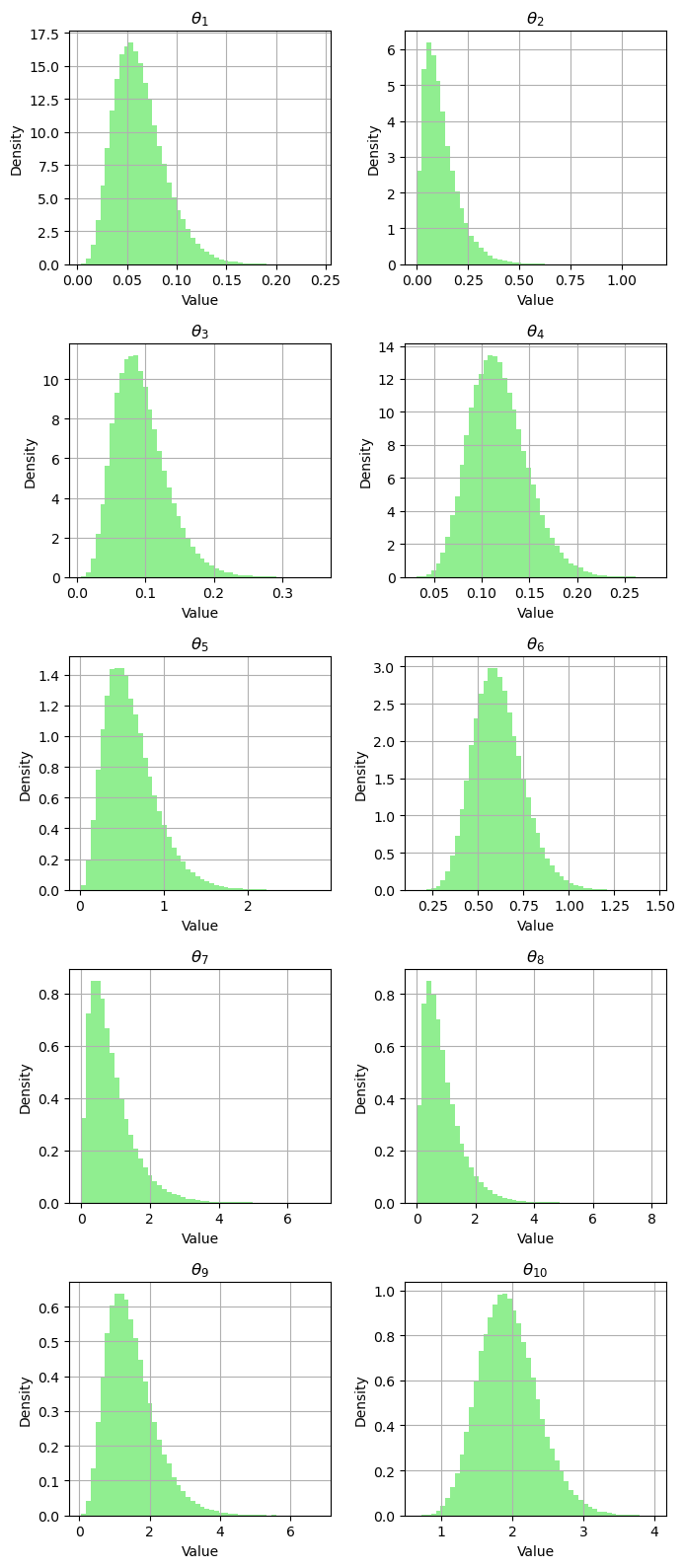
# Create histograms for thetas
fig, axes = plt.subplots(5, 2, figsize=(7, 16))

for i, ax in enumerate(axes.flatten()):
    ax.grid(True)
    ax.hist(thetas[:, i], color="lightgreen", density=True, bins=50)
    ax.set_title(r"$\theta_{" + f"{i+1}" + r"}$")
    ax.set_xlabel(f"Value")
    ax.set_ylabel(f"Density")

plt.tight_layout()

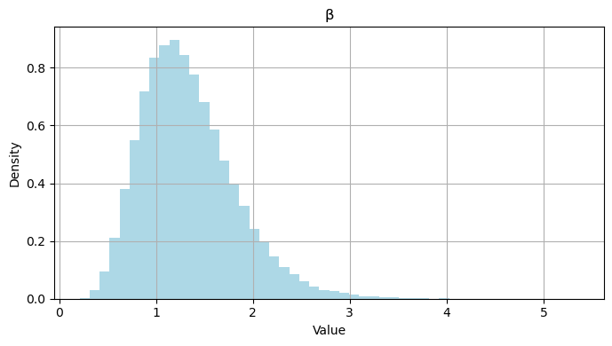
# Create a histogram for beta
fig2, ax2 = plt.subplots(1, 1, figsize=(7, 4))

ax2.grid(True)
ax2.hist(betas, color="lightblue", density=True, bins=50)
ax2.set_title("β")
ax2.set_xlabel("Value")
ax2.set_ylabel("Density")

plt.tight_layout()
plt.show()

means:
θ_1 : 0.0628
θ_2 : 0.1184
θ_3 : 0.0934
θ_4 : 0.1180
θ_5 : 0.6104
θ_6 : 0.6105
θ_7 : 0.8710
θ_8 : 0.8710
θ_9 : 1.4827
θ_10 : 1.9496
β: 1.3367

Now for the PyMC model:

with pm.Model() as m:
    times = pm.ConstantData("times", t)
    data = pm.ConstantData("data", X)

    beta = pm.Gamma("beta", alpha=c, beta=d)
    theta = pm.Gamma("theta", alpha=d, beta=beta, shape=n)
    rate = pm.Deterministic("rate", theta * times)

    likelihood = pm.Poisson("likelihood", mu=rate, observed=data)

    # start sampling
    trace = pm.sample(5000)

Show code cell output Hide code cell output

Auto-assigning NUTS sampler...
Initializing NUTS using jitter+adapt_diag...
Multiprocess sampling (4 chains in 4 jobs)
NUTS: [beta, theta]

100.00% [24000/24000 00:02<00:00 Sampling 4 chains, 0 divergences]

Sampling 4 chains for 1_000 tune and 5_000 draw iterations (4_000 + 20_000 draws total) took 3 seconds.

az.summary(trace, var_names=["~rate"])

	mean	sd	hdi_3%	hdi_97%	mcse_mean	mcse_sd	ess_bulk	ess_tail	r_hat
beta	1.336	0.489	0.496	2.235	0.003	0.002	28254.0	16048.0	1.0
theta[0]	0.063	0.026	0.020	0.112	0.000	0.000	32410.0	13799.0	1.0
theta[1]	0.118	0.083	0.005	0.270	0.000	0.000	29059.0	13169.0	1.0
theta[2]	0.093	0.038	0.028	0.163	0.000	0.000	33616.0	12846.0	1.0
theta[3]	0.118	0.030	0.064	0.176	0.000	0.000	32213.0	13436.0	1.0
theta[4]	0.615	0.309	0.129	1.195	0.002	0.001	31105.0	12634.0	1.0
theta[5]	0.610	0.134	0.368	0.866	0.001	0.001	35250.0	15216.0	1.0
theta[6]	0.868	0.650	0.020	2.044	0.004	0.003	27288.0	14224.0	1.0
theta[7]	0.867	0.643	0.017	2.004	0.004	0.003	26571.0	13272.0	1.0
theta[8]	1.485	0.698	0.336	2.769	0.004	0.003	31306.0	14821.0	1.0
theta[9]	1.949	0.413	1.208	2.721	0.002	0.002	33359.0	14035.0	1.0

Compare to BUGS results:

	mean	sd	MC_error	val2.5pc	median	val97.5pc	start	sample
beta	1.34	0.486	0.002973	0.5896	1.271	2.466	1001	50000
theta[1]	0.06261	0.02552	1.11E-04	0.02334	0.05914	0.1217	1001	50000
theta[2]	0.118	0.08349	3.69E-04	0.01431	0.09888	0.3296	1001	50000
theta[3]	0.09366	0.03829	1.71E-04	0.03439	0.08842	0.1828	1001	50000
theta[4]	0.1178	0.03048	1.47E-04	0.06595	0.115	0.1848	1001	50000
theta[5]	0.6116	0.3097	0.001409	0.1632	0.5589	1.361	1001	50000
theta[6]	0.6104	0.1366	6.45E-04	0.3705	0.6001	0.9058	1001	50000
theta[7]	0.8686	0.6494	0.003059	0.101	0.7124	2.537	1001	50000
theta[8]	0.8692	0.6481	0.003354	0.09784	0.7117	2.513	1001	50000
theta[9]	1.478	0.6897	0.00351	0.4705	1.367	3.128	1001	50000
theta[10]	1.944	0.4133	0.002022	1.223	1.916	2.83	1001	50000

%load_ext watermark
%watermark -n -u -v -iv -p pytensor

Last updated: Sun Aug 27 2023

Python implementation: CPython
Python version       : 3.11.4
IPython version      : 8.14.0

pytensor: 2.14.2

matplotlib: 3.7.2
numpy     : 1.24.4
arviz     : 0.16.1
pymc      : 5.7.1