16. Prior Sample Size

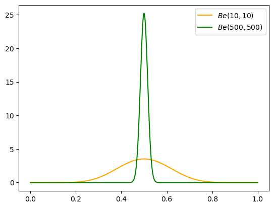
In lesson 7, when discussing different beta priors, the professor decided on \(Be(500, 500)\) as a realistic prior for a fair coin. But how would you decide between that and, say, \(Be(10, 10)\)? Both have a mean of \(.5\), but one is much stronger.

Show code cell source Hide code cell source

import numpy as np
from scipy.stats import beta
import matplotlib.pyplot as plt

xx = np.linspace(0, 1, 10000)
pdf_10 = beta.pdf(xx, 10, 10)
pdf_500 = beta.pdf(xx, 500, 500)

fig, ax = plt.subplots()

ax.plot(xx, pdf_10, color='orange', label='$Be(10, 10)$')
ax.plot(xx, pdf_500, color='green', label='$Be(500, 500)$')

ax.legend()
plt.show()

Effective sample size, as defined in the lecture, is an informal measure of the strength of a prior as it interacts with a particular likelihood to contribute to the posterior.

Warning

Effective sample size has another, more common meaning in a Bayesian context. From the Stan docs, “The amount by which autocorrelation within the chains increases uncertainty in estimates can be measured by effective sample size (ESS).” This is a totally unrelated use of the term, so don’t get them confused!

So if we’re using a beta-binomial conjugate model, we would say the ESS of \(Be(10, 10)\) is \(\alpha + \beta = 20\), while \(Be(500, 500)\) is \(1000\).

We’ve had questions about how the Normal-Gamma ESS was calculated on the last slide. I believe this is the reasoning: when you define the Normal distribution with precision and have a Gamma prior, the (conjugate) posterior is \(Gamma\left(\alpha + n/2, \beta + 1/2 \cdot \sum_{i=1}^{n} (x_i - n)^2\right)\), so the mean is \(\frac{\alpha + n/2}{\beta + 1/2 \cdot \sum_{i=1}^{n} (x_i - n)^2}\). Then Professor Vidakovic is informally comparing prior mean to posterior mean:

\[\frac{\alpha}{\beta} \rightarrow \frac{\alpha + n/2}{\beta + 1/2 \cdot \sum_{i=1}^{n} (x_i - n)^2} \rightarrow ESS = 2\alpha\]

Spiegelhalter’s categories and current recommendations

The professor mentions three different types of priors: vague, skeptical, and enthusiastic [Spiegelhalter et al., 1994]. These are similar to the five categories mentioned in the Stan Prior Choice Recommendations.

Both Stan and PyMC developers recommend prior predictive checks for your models. When combined with visualizations, these can help you check how realistic your priors are.