import matplotlib.pyplot as plt
import numpy as np
from tqdm.auto import tqdm
11. Normal-Cauchy Gibbs Sampler*#
Adapted from Unit 5: norcaugibbs.m.
Normal-Cauchy model#
Our model is:
\[\begin{split}
\begin{align*}
X|\theta &\sim \mathcal{N}(\theta, 1)\\
\theta &\sim \mathcal{Ca}(0,1) \\
\end{align*}
\end{split}\]
The problem is there’s only one parameter, \(\theta\), to simulate. The professor extends the model with the following property of the Cauchy distribution:
\[\begin{split}
\begin{align*}
\theta \,|\, \lambda &\sim \mathcal{N}\left(\mu, \frac{\tau^2}{\lambda}\right) \\
\lambda &\sim \text{Ga}\left(\frac{1}{2}, \frac{1}{2}\right) \\
\end{align*}
\end{split}\]
which makes our full model:
\[\begin{split}
\begin{align*}
X|\theta &\sim \mathcal{N}\left(\theta, 1\right)\\
\theta \,|\, \lambda &\sim \mathcal{N}\left(\mu, \frac{\tau^2}{\lambda}\right) \\
\lambda &\sim \text{Ga}\left(\frac{1}{2}, \frac{1}{2}\right) \\
\end{align*}
\end{split}\]
You can read more about this parameter expansion approach here.
The lecture slide says we’re looking for \(\delta(2)\). The lecture doesn’t really clarify that notation, but in the code \(x=2\) as our sole datapoint, so that must be what the professor meant.
The full conditionals are:
\[\begin{align*}
\theta | \lambda, X &\sim \mathcal{N}\left(\frac{\tau^2 x + \lambda \sigma^2 \mu}{\tau^2 + \lambda \sigma^2}, \frac{\tau^2 \sigma^2}{\tau^2 + \lambda \sigma^2}\right)
\end{align*}\]
\[\begin{align*}
\lambda | \theta, X &\sim \text{Exp}\left(\frac{\tau^2 + (\theta - \mu)^2}{2\tau^2}\right)
\end{align*}\]
rng = np.random.default_rng(1)

obs = 100000
burn = 1000

# params
x = 2
sigma2 = 1
tau2 = 1
mu = 0

# inits
theta = 0
lam = 1

thetas = np.zeros(obs)
lambdas = np.zeros(obs)

randn = rng.standard_normal(obs)

for i in tqdm(range(obs)):
    d = tau2 + lam * sigma2
    theta = (tau2 / d * x + lam * sigma2 / d * mu) + np.sqrt(tau2 * sigma2 / d) * randn[
        i
    ]
    lam = rng.exponential(1 / ((tau2 + (theta - mu) ** 2) / (2 * tau2)))

    thetas[i] = theta
    lambdas[i] = lam

thetas = thetas[burn:]
lambdas = lambdas[burn:]
Show code cell output
print(f"{np.mean(thetas)=}")
print(f"{np.var(thetas)=}")
print(f"{np.mean(lambdas)=}")
print(f"{np.var(lambdas)=}")
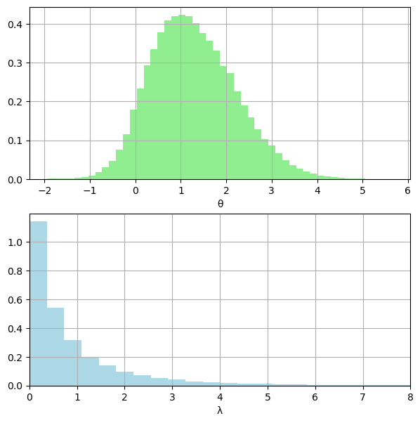
# posterior densities
fig, (ax1, ax2) = plt.subplots(2, 1, figsize=(7, 7))
ax1.grid(True)
ax1.hist(thetas, color="lightgreen", density=True, bins=50)
ax1.set_xlabel("θ")
ax2.grid(True)
ax2.hist(lambdas, color="lightblue", density=True, bins=50)
ax2.set_xlabel("λ")
ax2.set_xlim(0, 8)
plt.show()
np.mean(thetas)=1.2810728558916804
np.var(thetas)=0.860464992070327
np.mean(lambdas)=0.9408560283549908
np.var(lambdas)=1.5703387617734375
%load_ext watermark
%watermark -n -u -v -iv
Last updated: Tue Aug 22 2023

Python implementation: CPython
Python version       : 3.11.4
IPython version      : 8.14.0

numpy     : 1.24.4
matplotlib: 3.7.2