import arviz as az
import matplotlib.pyplot as plt
import pymc as pm
from pymc.math import invlogit
17. eBay Purchase Example*#
This example shows some of the effects different priors can have on your results.
From unit 4: eBay.odc.
Problem statement#
You’ve decided to purchase a new Orbital Shaking Incubator for your research lab on eBay.
Two sellers are offering this item for the same price, both with free shipping.
The sellers in question are:
Seller A: 95% positive feedback from 100 sales.
Seller B: 100% positive feedback from just 3 sales.
We assume that all 103 responders are different, unrelated customers, to avoid dependent responses.
From which seller should you order?
That depends on your priors!
Note
I changed labels 1 and 2 in the model to A and B to align with the problem definition.
# data
pos_A = 95
tot_A = 100

tot_B = 3
pos_B = 3
# lots of problems in PyMC 4, probably need to redo later
with pm.Model() as m:
    # priors
    priors_A = (
        pm.Beta("uniform_A", alpha=1, beta=1),
        pm.Beta("jeffrey_A", alpha=0.5, beta=0.5),
        pm.Beta("informative_A", alpha=30, beta=2),
        pm.Deterministic(
            "zellner_A", invlogit(pm.Uniform("ign_A", lower=-1000, upper=1000))
        ),
        pm.LogitNormal("norm_A", mu=3, sigma=1),
    )

    priors_B = (
        pm.Beta("uniform_B", alpha=1, beta=1),
        pm.Beta("jeffrey_B", alpha=0.5, beta=0.5),
        pm.Beta("informative_B", alpha=2.9, beta=0.1),
        pm.Deterministic(
            "zellner_B", invlogit(pm.Uniform("ign_B", lower=-1000, upper=1000))
        ),
        pm.LogitNormal("norm_B", mu=3, sigma=1),
    )

    # likelihoods
    for A, B in zip(priors_A, priors_B):
        prior_type = A.name.strip("_A")

        pm.Binomial("y_" + A.name, n=tot_A, p=A, observed=pos_A)
        pm.Binomial("y_" + B.name, n=tot_B, p=B, observed=pos_B)

        pm.Deterministic("diff_" + prior_type, A - B)

    # start sampling
    trace = pm.sample(4000, tune=2000, target_accept=0.9)
Show code cell output
Auto-assigning NUTS sampler...
Initializing NUTS using jitter+adapt_diag...
Multiprocess sampling (4 chains in 4 jobs)
NUTS: [uniform_A, jeffrey_A, informative_A, ign_A, norm_A, uniform_B, jeffrey_B, informative_B, ign_B, norm_B]
Sampling 4 chains for 2_000 tune and 4_000 draw iterations (8_000 + 16_000 draws total) took 233 seconds.
There were 1068 divergences after tuning. Increase `target_accept` or reparameterize.
PyMC is deeply unhappy with some of these models but the results are the same as BUGS, so I’m going to leave well enough alone.
az.summary(trace, var_names=["~ign_A", "~ign_B"], hdi_prob=0.95)
| mean | sd | hdi_2.5% | hdi_97.5% | mcse_mean | mcse_sd | ess_bulk | ess_tail | r_hat | |
|---|---|---|---|---|---|---|---|---|---|
| uniform_A | 0.941 | 0.024 | 0.895 | 0.982 | 0.000 | 0.000 | 5311.0 | 4935.0 | 1.0 |
| jeffrey_A | 0.945 | 0.023 | 0.900 | 0.984 | 0.000 | 0.000 | 4856.0 | 4704.0 | 1.0 |
| informative_A | 0.947 | 0.019 | 0.908 | 0.981 | 0.000 | 0.000 | 5365.0 | 5167.0 | 1.0 |
| norm_A | 0.950 | 0.020 | 0.910 | 0.984 | 0.000 | 0.000 | 5456.0 | 5831.0 | 1.0 |
| uniform_B | 0.802 | 0.163 | 0.472 | 1.000 | 0.002 | 0.002 | 4677.0 | 3701.0 | 1.0 |
| jeffrey_B | 0.874 | 0.150 | 0.550 | 1.000 | 0.002 | 0.001 | 3550.0 | 2841.0 | 1.0 |
| informative_B | 0.983 | 0.048 | 0.902 | 1.000 | 0.000 | 0.000 | 2229.0 | 1282.0 | 1.0 |
| norm_B | 0.943 | 0.052 | 0.842 | 0.998 | 0.001 | 0.001 | 5079.0 | 6250.0 | 1.0 |
| zellner_A | 0.951 | 0.021 | 0.908 | 0.987 | 0.000 | 0.000 | 4274.0 | 3839.0 | 1.0 |
| zellner_B | 1.000 | 0.004 | 1.000 | 1.000 | 0.000 | 0.000 | 9338.0 | 16000.0 | 1.0 |
| diff_uniform | 0.140 | 0.165 | -0.089 | 0.486 | 0.002 | 0.002 | 4997.0 | 5242.0 | 1.0 |
| diff_jeffrey | 0.071 | 0.152 | -0.111 | 0.405 | 0.002 | 0.001 | 4877.0 | 6837.0 | 1.0 |
| diff_informative | -0.036 | 0.052 | -0.110 | 0.059 | 0.000 | 0.000 | 7083.0 | 8247.0 | 1.0 |
| diff_zellner | -0.049 | 0.022 | -0.092 | -0.013 | 0.000 | 0.000 | 4339.0 | 3859.0 | 1.0 |
| diff_norm | 0.006 | 0.056 | -0.080 | 0.123 | 0.001 | 0.001 | 5022.0 | 7143.0 | 1.0 |
The results are pretty close to the professor’s BUGS results:
mean |
sd |
MC_error |
val2.5pc |
median |
val97.5pc |
|
|---|---|---|---|---|---|---|
diffps[1] |
0.1417 |
0.1649 |
4.93E-04 |
-0.06535 |
0.1018 |
0.5448 |
diffps[2] |
0.06921 |
0.1485 |
4.63E-04 |
-0.08247 |
0.01423 |
0.4774 |
diffps[3] |
-0.03623 |
0.05252 |
1.70E-04 |
-0.09355 |
-0.04494 |
0.1144 |
diffps[4] |
-0.05004 |
0.02177 |
7.02E-05 |
-0.1003 |
-0.04712 |
-0.0164 |
diffps[5] |
0.00658 |
0.05593 |
1.73E-04 |
-0.06808 |
-0.005543 |
0.1526 |
p1[1] |
0.9412 |
0.02319 |
7.40E-05 |
0.8882 |
0.9442 |
0.9778 |
p1[2] |
0.9456 |
0.02235 |
7.13E-05 |
0.8944 |
0.9485 |
0.9808 |
p1[3] |
0.9471 |
0.01937 |
6.09E-05 |
0.9031 |
0.9493 |
0.9782 |
p1[4] |
0.9499 |
0.02169 |
7.04E-05 |
0.8997 |
0.9529 |
0.9836 |
p1[5] |
0.9498 |
0.01973 |
5.96E-05 |
0.9043 |
0.9525 |
0.9804 |
p2[1] |
0.7995 |
0.1632 |
4.89E-04 |
0.3982 |
0.8402 |
0.9938 |
p2[2] |
0.8764 |
0.1468 |
4.56E-04 |
0.4694 |
0.9336 |
0.9999 |
p2[3] |
0.9833 |
0.04892 |
1.58E-04 |
0.8344 |
0.9999 |
1 |
p2[4] |
1 |
0.001891 |
5.84E-06 |
1 |
1 |
1 |
p2[5] |
0.9432 |
0.05234 |
1.66E-04 |
0.7986 |
0.9592 |
0.9935 |
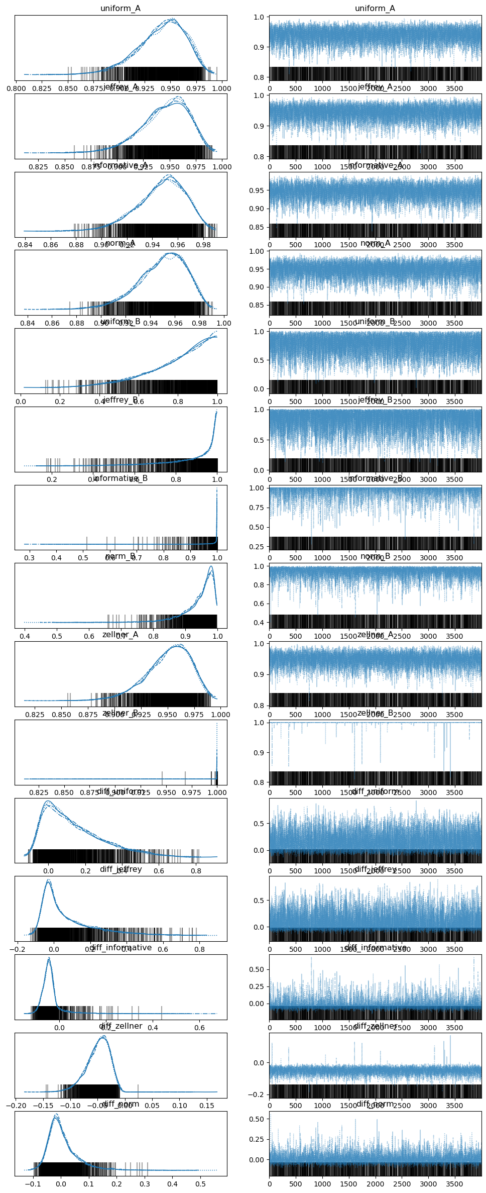
az.plot_trace(trace, var_names=["~ign_A", "~ign_B"])
plt.show()
%load_ext watermark
%watermark -n -u -v -iv -p pytensor
Last updated: Mon Jul 10 2023

Python implementation: CPython
Python version       : 3.11.0
IPython version      : 8.9.0

pytensor: 2.11.1

arviz     : 0.15.1
pymc      : 5.3.0
matplotlib: 3.6.3