import arviz as az
import matplotlib.pyplot as plt
import numpy as np
import pymc as pm

%load_ext lab_black

7. Ten Coin Flips Revisited: Beta Plots*

From Unit 4: betaplots.m.

The professor goes back to the Ten Coin Flips example from Unit 2. A coin was flipped ten times, coming up tails each time. We have no reason to believe it is a trick coin. Frequentist methods came up with an estimate of \(p = 0\) for the probability of the next flip, since they depend only on the data we’ve collected so far. But when we put a uniform prior on \(p\), we came up with a posterior probability of \(1/12\).

In this lecture, we take a look at the more expressive Beta distribution. Describing this distribution are the shape parameters \(\alpha\) and \(\beta\), which interact to define the mean at \(\frac{\alpha}{\alpha+\beta}\). Beta priors are conjugate with the binomial likelihood, so they fit naturally here.

See also

Example 8.4, Vidakovic [2017] p. 341.

First, take a look at some plots of various beta distributions.

Show code cell source Hide code cell source

params = [
    (0.5, 0.5),
    (1, 1),
    (2, 2),
    (10, 10),
    (1, 5),
    (1, 0.4),
    (3, 5),
    (50, 30),
    (5000, 3000),
    (500, 500),
]


def beta_dist(α, β, n):
    """
    Return n samples from a Beta(α, β) dist. along with a name string.
    """
    name = f"{α=}, {β=}"
    return pm.draw(pm.Beta.dist(α, β), n), name


n = 100000
distributions = [beta_dist(α, β, n) for α, β in params]

fig, ax = plt.subplots(nrows=5, ncols=2, figsize=(8, 22), sharex="col")

for i, dist in enumerate(distributions):
    plt.subplot(5, 2, i + 1, autoscalex_on=False)
    az.plot_dist(dist[0], figsize=(2, 2))
    plt.title(dist[1])

plt.xlim(0, 1)
plt.show()

/var/folders/pm/9z29qnf508bc1v6q8fksblm40000gn/T/ipykernel_27241/1374941424.py:26: MatplotlibDeprecationWarning: Auto-removal of overlapping axes is deprecated since 3.6 and will be removed two minor releases later; explicitly call ax.remove() as needed.
  plt.subplot(5, 2, i + 1, autoscalex_on=False)

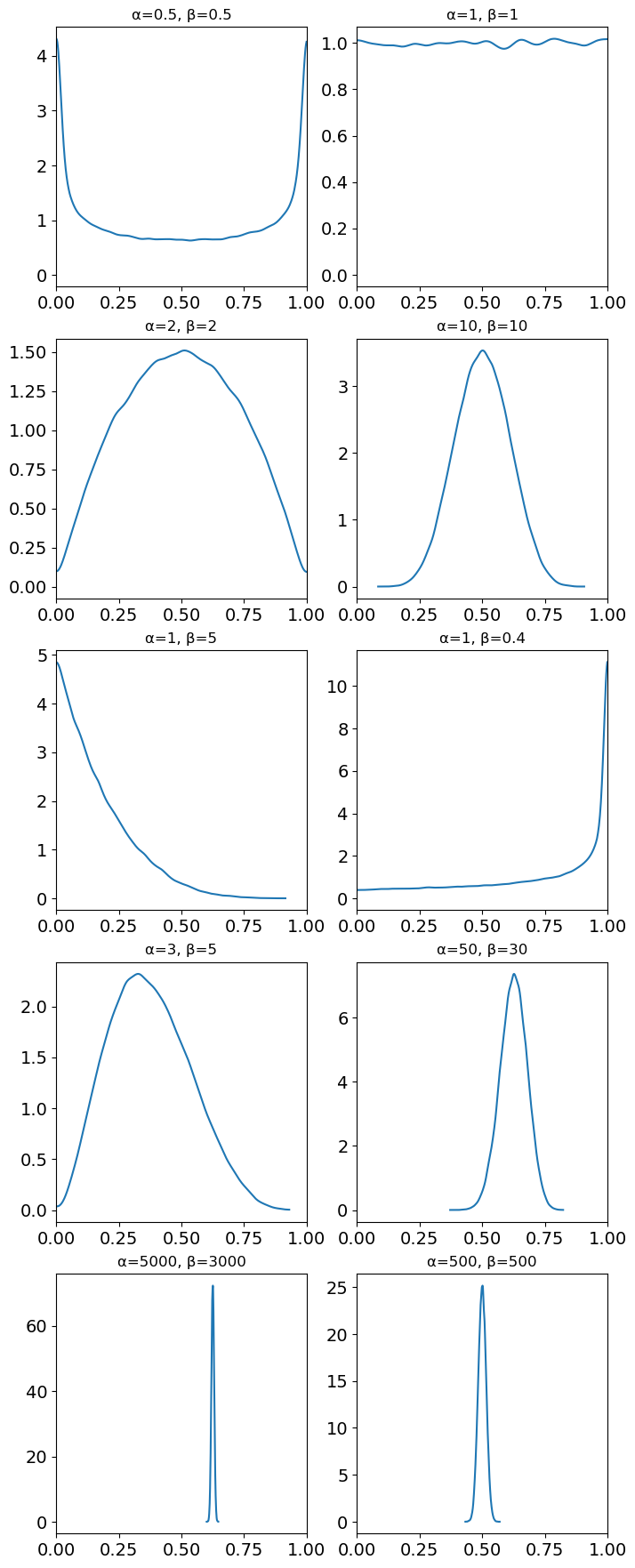
The professor decides on \(Be(500, 500)\) as a realistic fair coin prior, with the density heavily concentrated at the mean of \(.50\). So our model looks like this:

\[\begin{split} \begin{align*} X | p &\sim Bin(10, p) \\ p &\sim Be(500, 500) \end{align*} \end{split}\]

We know \(x=0, n=10\). Then:

\[\begin{split} \begin{align*} p \mid X &\sim Be(x + \alpha, n - x + \beta) \\ &\sim Be(500, 10 + 500) \\ &\sim Be(500, 510) \end{align*} \end{split}\]

Our Bayes estimator is \(\frac{\alpha}{\alpha+\beta} = \frac{500}{500+510} = .495\). So with this extremely strong prior expressing our belief that the coin was fair, ten tails-up flips in a row barely nudges our posterior belief. Try it with some different priors and see what you get!

You’ll notice this doesn’t look quite the same as in the conjugate table. That’s because the conjugate table version is more general: there, \(m\) is the same as \(n\) in this example. Then the table version’s \(n\) is the number of binomial experiments. Say you had run 3 experiments of 10 flips each. Then \(m\) would be 10, and \(n\) would be 3. You would have 3 \(x\) values, one for each experiment.

See also

Check out https://colcarroll.github.io/updating_beta/ for a nice visualization of the beta distribution.

%load_ext watermark
%watermark -n -u -v -iv -p pytensor

Last updated: Sat Mar 18 2023

Python implementation: CPython
Python version       : 3.11.0
IPython version      : 8.9.0

pytensor: 2.10.1

pymc      : 5.1.1
arviz     : 0.14.0
numpy     : 1.24.2
matplotlib: 3.6.3